Iris数据集训练感知机模型

感知机

基于MCP神经元模型,Frank Rosenblatt发表了第一个感知机学习规则(F.Rosenblatt, The Perceptron, a Perceiving and Recognizing Automaton. Cornell Aeronautical Laboratory, 1957)。
基于此感知机规则,Rosenblatt提出了能够自动学习最优权重参数的算法,权重即输入特征的系数。在监督学习和分类任务语境中,上面提到的算法还能够用于预测一个样本是属于类别A还是类别B。

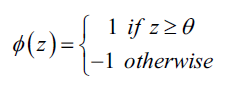
更准确的描述是,我们可以将上面提到的样本属于哪一个类别这个问题称之为二分类问题(binary classification task),我们将其中涉及到的两个类别记作1(表示正类)和-1(表示负类)。我们再定义一个称为激活函数(activation function) $\phi(z)$,激活函数接收一个输入向量$x$和相应的权重向量$w$的线性组合,其中$z$也被称为网络输入 $z=w_1x_1+\ldots+w_mx_m$ :

此时,如果某个样本$x^{(i)}$的激活值,即$\phi(z)$大于事先设置的阈值$\theta$,我们就说样本$x^{(i)}$属于类别1,否则属于类别-1。

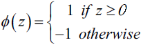
在感知机学习算法中,激活函数$\phi(z)$的形式非常简单,仅仅是一个单位阶跃函数(也被称为Heaviside阶跃函数):

为了推导简单,我们可以将阈值$\theta$挪到等式左边并且额外定义一个权重参数$w_0=-\theta$, 这样我们可以对$z$给出更加紧凑的公式$z=w_0x_0+w_1x_1+…+w_mx_m=w^Tx$,此时

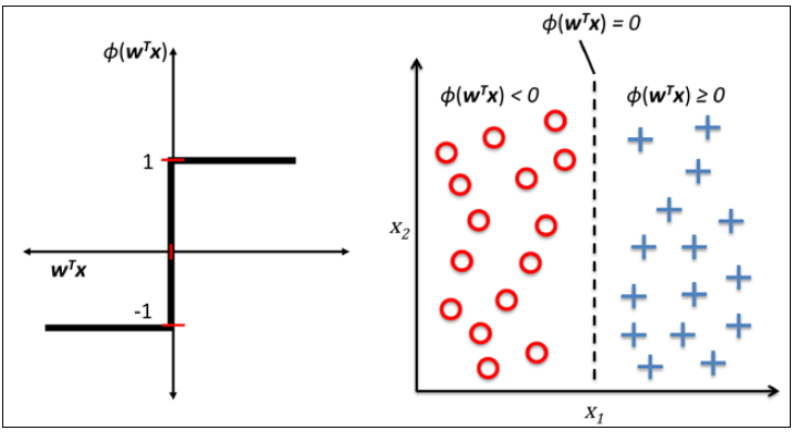
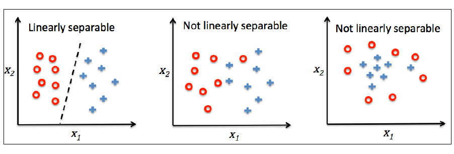
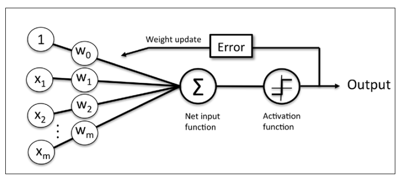
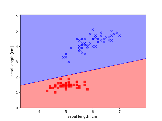
下面左图描述了感知机的激活函数怎样将网络输入$z=w^Tx$压缩到二元输出(-1,1),右图描述了感知机如何区分两个线性可分的类别。

不论MCP神经元还是Rosenblatt的阈值感知机模型,他们背后的idea都是试图使用简单的方法来模拟大脑中单个神经元的工作方式:要么传递信号要么不传递。因此,Rosenblatt最初的感知机规则非常简单,步骤如下:

  • 将权重参数初始化为0或者很小的随机数。
  • 对于每一个训练集样本$x^{(i)}$,执行下面的步骤:
    • 计数输出值 $\hat{y}$.
    • 更新权重参数.

此处的输出值就是单位阶跃函数预测的类别(1,-1),参数向量$w$中的每个$w_j$的更新过程可以用数学语言表示为:

其中 $\Delta w_j$,用于更新权重$w_j$,在感知机算法中的计算公式为:

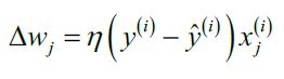
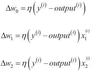
其中$\eta$ 称为学习率(learning rate), 是一个介于0.0和1.0之间的常数,$y^{(i)}$是第i个训练样本的真实类别,$\hat{y}^{(i)}$是对第i个训练样本的预测类别。 权重向量中的每一个参数 $w_j$ 是同时被更新的,这意味着在所有的 $\Delta w_j$计算出来以前不会重新计算 $\hat{y}^{(i)}$。具体地,对于一个二维数据集,我们可以将更新过程写为:

感知机算法仅在两个类别确实线性可分并且学习率充分小的情况下才能保证收敛。如果两个类别不能被一个线性决策界分开,我们可以设置最大训练集迭代次数(epoch)或者可容忍的错误分类样本数 来停止算法的学习过程。

在进入下一节的代码实现之前,我们来总结一下感知机的要点:

感知机接收一个样本输入x,然后将其和权重w结合,计算网络输入z。z接着被传递给激活函数,产生一个二分类输出-1或1作为预测的样本类别。在整个学习阶段,输出用于计算预测错误率(y-$\hat{y}$)和更新权重参数。

python 实现感知机算法

  • perceptron.py
1
2
3
4
5
6
7
8
9
10
11
12
13
14
15
16
17
18
19
20
21
22
23
24
25
26
27
28
29
30
31
32
33
34
35
36
37
38
39
40
41
42
43
44
45
46
47
48
49
50
51
52
53
54
55
56
57
58
59
60
61
62
63
64
65
66
67
68
69
70
71
#!/usr/bin/env python
# -*- coding: utf-8 -*-

"""
@author: janes
@file: perceptron.py
@time: 2017/4/7 13:45
"""

import numpy as np


class Perceptron(object):
"""Perceptron classifier.

Parameters
------------
eta:float
Learning rate (between 0.0 and 1.0)
n_iter:int
Passes over the training dataset.

Attributes
-------------
w_: 1d-array
Weights after fitting.
errors_: list
Numebr of misclassifications in every epoch.
"""

def __init__(self, eta=0.01, n_iter=10):
self.eta = eta
self.n_iter = n_iter

def fit(self, X, y):
"""Fit training data.

Parameters
------------
X: {array-like}, shape=[n_samples, n_features]
Training vectors, where n_samples is the number of samples
and n_featuers is the number of features.
y: array-like, shape=[n_smaples]
Target values.

Returns
----------
self: object
"""

# Add w_0
self.w_ = np.zeros(1 + X.shape[1])
self.errors_ = []

for _ in range(self.n_iter):
errors = 0
for xi, target in zip(X, y):
update = self.eta * (target - self.predict(xi))
self.w_[1:] += update * xi
self.w_[0] += update
errors += int(update != 0.0)
self.errors_.append(errors)
return self

def net_input(self, X):
"""Calculate net input"""
return np.dot(X, self.w_[1:]) + self.w_[0]

def predict(self, X):
"""Return class label after unit step"""
return np.where(self.net_input(X) >= 0.0, 1, -1)

初始化一个新的Perceptron对象,并且对学习率eta和迭代次数n_iter赋值,fit方法先对权重参数初始化,然后对训练集中每一个样本循环,根据感知机算法对权重进行更新。类别通过predict方法进行预测。除此之外,self.errors_ 还记录了每一轮中误分类的样本数,有助于接下来我们分析感知机的训练过程。

Iris数据集训练感知机算法

数据集

使用UCI机器学习数据库提供的Iris数据集, UCI网址: http://archive.ics.uci.edu/ml/, UCI机器学习库包含超过350个数据集,其标签分类包括域、目的(分类、回归)。

以Iris为例介绍一下数据集:

ucidata/iris中有三个文件:Index, iris.data, iris.names

index为文件夹目录,列出了本文件夹里的所有文件

iris.data为iris数据文件,内容如下:

1
2
3
4
5
6
7
8
9
5.1,3.5,1.4,0.2,Iris-setosa
4.9,3.0,1.4,0.2,Iris-setosa
……
7.0,3.2,4.7,1.4,Iris-versicolor
6.4,3.2,4.5,1.5,Iris-versicolor
……
6.3,3.3,6.0,2.5,Iris-virginica
5.8,2.7,5.1,1.9,Iris-virginica
7.1,3.0,5.9,2.1,Iris-virginica

如上,属性直接以逗号隔开,中间没有空格(5.1,3.5,1.4,0.2,),最后一列为本行属性对应的值,即决策属性Iris-setosa

iris.names介绍了irir数据的一些相关信息,如数据标题、数据来源、以前使用情况、最近信息、实例数目、实例的属性等,如下所示部分:

1
2
3
4
5
6
7
8
9
10
11
……
Attribute Information:

1. sepal length in cm
2. sepal width in cm
3. petal length in cm
4. petal width in cm
5. class:
-- Iris Setosa
-- Iris Versicolour
-- Iris Virginica

训练

我们仅使用Iris中Setosa和Versicolor两种花的数据,抽取出前100条样本,这正好是Setosa和Versicolor对应的样本,我们将Versicolor对应的数据作为类别1,Setosa对应的作为-1。对于特征,我们抽取出sepal length和petal length两维度特征。

  • test.py
1
2
3
4
5
6
7
8
9
10
11
12
13
14
15
16
17
18
19
20
21
22
23
24
25
26
27
28
29
30
31
32
33
34
35
36
37
38
39
40
41
42
43
44
45
46
47
48
49
50
51
52
53
54
55
56
57
58
59
60
61
62
63
64
65
66
67
68
69
70
#!/usr/bin/env python
# -*- coding: utf-8 -*-

"""
@author: janes
@file: perceptron.py
@time: 2017/4/7 13:45
"""

import numpy as np
import matplotlib.pyplot as plt
from matplotlib.colors import ListedColormap
import pandas as pd
from perceptron import Perceptron


def plot_x(X):
plt.scatter(X[:50, 0], X[:50, 1], color='red', marker='o', label='setosa')
plt.scatter(X[50:, 0], X[50:, 1], color='blue', marker='x', label='versicolor')
plt.xlabel('petal length')
plt.ylabel('sepal length')
plt.legend(loc='upper left')
plt.show()


def plot_decision_region(X, y, classifier, resolution=0.02):
markers = ('s', 'x', 'o', '^', 'v')
colors = ('red', 'blue', 'lightgreen', 'gray', 'cyan')
cmap = ListedColormap(colors[:len(np.unique(y))])

x1_min, x1_max = X[:, 0].min()-1, X[:, 0].max() + 1
x2_min, x2_max = X[:, 1].min()-1, X[:, 1].max() + 1

xx1, xx2 = np.meshgrid(np.arange(x1_min, x1_max, resolution),
np.arange(x2_min, x2_max, resolution))
Z = classifier.predict(np.array([xx1.ravel(), xx2.ravel()]).T)
Z = Z.reshape(xx1.shape)

plt.contourf(xx1, xx2, Z, alpha=0.4, cmap=cmap)
plt.xlim(xx1.min(), xx1.max())
plt.ylim(xx2.min(), xx2.max())

for idx, cl in enumerate(np.unique(y)):
plt.scatter(x=X[y == cl, 0], y=X[y == cl, 1], alpha=0.8, c=cmap(idx),
marker=markers[idx], label=cl)

plt.xlabel('sepal length [cm]')
plt.ylabel('petal length [cm]')
plt.show()


def plot_misclassifications(classifier):
plt.plot(range(1, len(classifier.errors_)+1), classifier.errors_, marker='o')
plt.xlabel('Epoches')
plt.ylabel('Numebr of misclassifications')
plt.show()


if __name__ == "__main__":
df = pd.read_csv('iris.data.csv', header=None)
y = df.iloc[0:100, 4].values
y = np.where(y == 'Iris-setosa', -1, 1)
X = df.iloc[0:100, [0, 2]].values

ppn = Perceptron(eta=0.1, n_iter=10)
ppn.fit(X, y)

# plot_x(X)
# plot_misclassifications(ppn)
plot_decision_region(X, y, ppn)

虽然对于Iris数据集,感知机算法表现的很完美,但是”收敛”一直是感知机算法中的一大问题。Frank Rosenblatt从数学上证明了只要两个类别能够被一个现行超平面分开,则感知机算法一定能够收敛。然而,如果数据并非线性可分,感知计算法则会一直运行下去,除非我们人为设置最大迭代次数n_iter

reference